11 Two slopes method
For a description of the two slopes method see [12].
This method is shown unless the software was compiled without Fortran support.
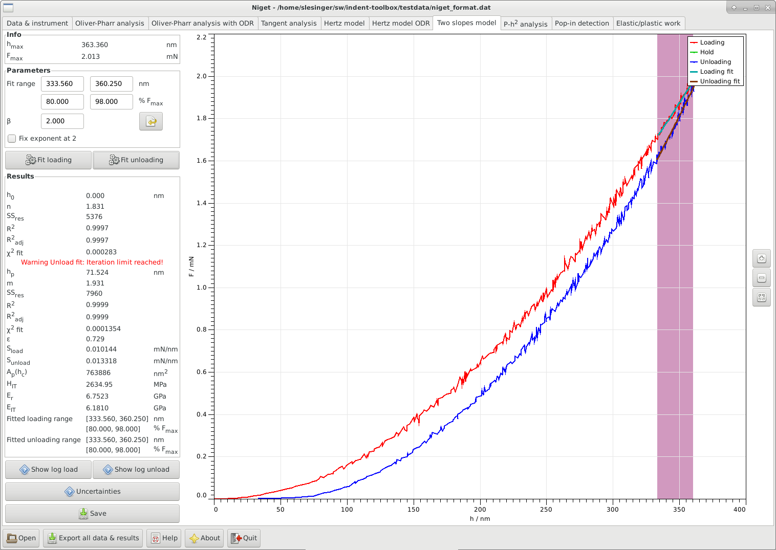
11.1 Window
The window consists of several blocks:
-
•
Info displays the maximum depth and force during the indentation
-
•
Parameters shows the selected range in nm and in % of the maximum force, and the correction
 .
.-
-
The fitting range can be selected either using the mouse or typing in the range entries. The range can be defined either in nm or in percent of the maximum force. It is often recommended to use the range 80–98 % F
 for the fit, see section 11.2.
 -
-
The parameter
accounts for any deviations from the axisymmetric case and is used in the calculation of the reduced modulus in equation (10).
Currently, the default value is no correction  . The value supplied by the user is saved in the settings and can be reset to its default value.
 -
-
Check box, whether or not the exponent of the loading curve should be fitted or fixed at the theoretical value 2, see 11.2.
-
-
-
•
Fit buttons for indepedent fitting of the loading and unloading curves, see section 11.2 for details of the calculation.
-
•
Results displays all results in the following order: the auxiliary depth parameter
 , the power
  of the power law loading function,
the residual depth
of the power law loading function,
the residual depth  , the power
  of the power law unloading function, the parameter
  ,
the loading slope
,
the loading slope  , the unloadingslope
  ,
the contact area
,
the contact area  , the indentation hardness
  , the contact modulus
  , the indentation modulus
  and the ranges used for the fitting procedures.
The variables are described in detail in section 11.2. Warnings are displayed if the fittings procedures failed.
and the ranges used for the fitting procedures.
The variables are described in detail in section 11.2. Warnings are displayed if the fittings procedures failed. -
•
Uncertainties show the uncertainty analysis window, see section 15.2.4.
-
•
Show log load Show the report about the fitting procedure of the loading curve in a separate window. The reports are saved to files fit.log.slopes.load.err and fit.log.slopes.load.rpt.
-
•
Show log unload Show the report about the fitting procedure of the unloading curve in a separate window. The reports are saved to files fit.log.slopes.unload.err and
fit.log.slopes.unload.rpt. -
•
Save save parameters and results to given file.
-
•
Graph display the unloading curve and the fitted curves. Stepwise zooming/unzooming can be performed by selecting a range with the mouse and pressing the Zoom/ Unzoom buttons. The graph is restored to its original size by the Restore button.
11.2 Procedure
The two slopes method combines the standard Oliver Pharr method and the quadratic loading curve to avoid the need of the contact area.
-
1.
Fit the upper part of the loading curve with a power law function
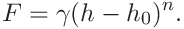
using orthogonal least squares as implemented in the package ODRPACK95 [13]. The range should be approx. 85–98 % F
. The exponent can be kept fixed at its theoretical value 2. -
2.
Fit the upper part of the unloading curve with a power law function
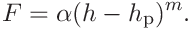
using orthogonal least squares as implemented in the package ODRPACK95 [13]. The range should be approx. 85–98 % F
. All three parameters are fitted. -
3.
The auxiliary parameter
is calculated from the power as in (6) -
4.
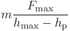
The slopes at the maximum depth are calculated as


(23) 
(24) -
5.
The contact area, indentation hardness and contact modulus are calculated as

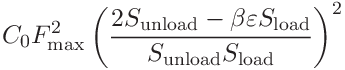
(25) 
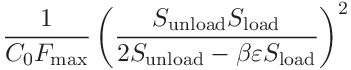
(26) 
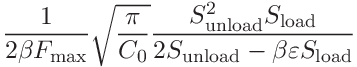
(27) with
 the coefficient of the
  term in the area calibration function and a geometric correction term. Currently, we use
  .
. -
6.
The indentation modulus can be calculated from (11)
![[LOGO]](data:image/png;base64,iVBORw0KGgoAAAANSUhEUgAAAAsAAAAOCAYAAAD5YeaVAAAAAXNSR0IArs4c6QAAAAZiS0dEAP8A/wD/oL2nkwAAAAlwSFlzAAALEwAACxMBAJqcGAAAAAd0SU1FB9wKExQZLWTEaOUAAAAddEVYdENvbW1lbnQAQ3JlYXRlZCB3aXRoIFRoZSBHSU1Q72QlbgAAAdpJREFUKM9tkL+L2nAARz9fPZNCKFapUn8kyI0e4iRHSR1Kb8ng0lJw6FYHFwv2LwhOpcWxTjeUunYqOmqd6hEoRDhtDWdA8ApRYsSUCDHNt5ul13vz4w0vWCgUnnEc975arX6ORqN3VqtVZbfbTQC4uEHANM3jSqXymFI6yWazP2KxWAXAL9zCUa1Wy2tXVxheKA9YNoR8Pt+aTqe4FVVVvz05O6MBhqUIBGk8Hn8HAOVy+T+XLJfLS4ZhTiRJgqIoVBRFIoric47jPnmeB1mW/9rr9ZpSSn3Lsmir1fJZlqWlUonKsvwWwD8ymc/nXwVBeLjf7xEKhdBut9Hr9WgmkyGEkJwsy5eHG5vN5g0AKIoCAEgkEkin0wQAfN9/cXPdheu6P33fBwB4ngcAcByHJpPJl+fn54mD3Gg0NrquXxeLRQAAwzAYj8cwTZPwPH9/sVg8PXweDAauqqr2cDjEer1GJBLBZDJBs9mE4zjwfZ85lAGg2+06hmGgXq+j3+/DsixYlgVN03a9Xu8jgCNCyIegIAgx13Vfd7vdu+FweG8YRkjXdWy329+dTgeSJD3ieZ7RNO0VAXAPwDEAO5VKndi2fWrb9jWl9Esul6PZbDY9Go1OZ7PZ9z/lyuD3OozU2wAAAABJRU5ErkJggg==)