Appendix A Data fitting
We use types of data fitting: the Deming fit for straight lines, the least squares fit of the 3/2 power and orthogonal distance regression [2] for power law functions.
A.1 Orthogonal distance regression
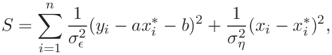
Orthogonal distance regression, also called generalized least squares regression, errors-in-variables models or measurement error models, attempts to tries to find the best fit taking into account errors in both x- and y- values. Assuming the relationship
| (60) |
where ![]() are parameters and
are parameters and ![]() and
and ![]() are the “true” values, without error, this leads to a minimization of the sum
are the “true” values, without error, this leads to a minimization of the sum
![\min_{\beta,\delta}\sum_{i=1}^{n}\left[\left(y_{i}-f(x_{i}+\delta;\beta)\right%
)^{2}+\delta_{i}^{2}\right]](mi/mi340.png) |
(61) |
which can be interpreted as the sum of orthogonal distances from the data points ![]() to the curve
to the curve ![]() .
It can be rewritten as
.
It can be rewritten as
![\min_{\beta,\delta,\varepsilon}\sum_{i=1}^{n}\left[\varepsilon_{i}^{2}+\delta_%
{i}^{2}\right]](mi/mi338.png) |
(62) |
subject to
| (63) |
This can be generalized to accomodate different weights for the datapoints and to higher dimensions
![\min_{\beta,\delta,\varepsilon}\sum_{i=1}^{n}\left[\varepsilon_{i}^{T}w^{2}_{%
\varepsilon}\varepsilon_{i}+\delta_{i}^{T}w^{2}_{\delta}\delta_{i}\right],](mi/mi339.png) |
where ![]() and
and ![]() are
are ![]() and
and ![]() dimensional vectors and
dimensional vectors and ![]() and
and ![]() are symmetric, positive diagonal matrices.
Usually the inverse uncertainties of the data points are chosen as weights.
We use the implementation ODRPACK [2].
are symmetric, positive diagonal matrices.
Usually the inverse uncertainties of the data points are chosen as weights.
We use the implementation ODRPACK [2].
There are different estimates of the covariance matrix of the fitted parameters ![]() .
Most of them are based on the linearization method which assumes that the nonlinear function can be adequately approximated at the solution by a linear model. Here,
we use an approximation where the covariance matrix associated with the parameter estimates is based
.
Most of them are based on the linearization method which assumes that the nonlinear function can be adequately approximated at the solution by a linear model. Here,
we use an approximation where the covariance matrix associated with the parameter estimates is based ![]() , where
, where ![]() is the Jacobian matrix of
the x and y residuals, weighted by the triangular matrix of the Cholesky factorization of the covariance matrix associated with the experimental data.
ODRPACK uses the following implementation [1]
is the Jacobian matrix of
the x and y residuals, weighted by the triangular matrix of the Cholesky factorization of the covariance matrix associated with the experimental data.
ODRPACK uses the following implementation [1]
![\hat{V}=\hat{\sigma}^{2}\left[\sum_{i=1}^{n}\frac{\partial f(x_{i}+\delta_{i};%
\beta)}{\partial\beta^{T}}w^{2}_{\varepsilon_{i}}\frac{\partial f(x_{i}+\delta%
_{i};\beta)}{\partial\beta}+\frac{\partial f(x_{i}+\delta_{i};\beta)}{\partial%
\delta^{T}}w^{2}_{\delta_{i}}\frac{\partial f(x_{i}+\delta_{i};\beta)}{%
\partial\delta}\right]](mi/mi336.png) |
(64) |
The residual variance ![]() is estimated as
is estimated as
![\hat{\sigma}^{2}=\frac{1}{n-p}\sum_{i=1}^{n}\left[\left(y_{i}-f(x_{i}+\delta;%
\beta)\right)^{T}w^{2}_{\varepsilon_{i}}\left(y_{i}-f(x_{i}+\delta;\beta)%
\right)+\delta_{i}^{T}w^{2}_{\delta_{i}}\delta_{i}\right]](mi/mi337.png) |
(65) |
where ![]() and
and ![]() are the optimized parameters,
are the optimized parameters,
A.2 Total least squares - Deming fit
The Deming fit is a special case of orthogonal regression which can be solved analytically. It seeks the best fit to a linear relationship between the x- and y-values
| (66) |
by minimizing the weighted sum of (orthogonal) distances of datapoints from the curve
 |
with respect to the parameters ![]() ,
, ![]() , and
, and ![]() .
The weights are the variances of the errors in the x-variable (
.
The weights are the variances of the errors in the x-variable (![]() ) and the y-variable (
) and the y-variable (![]() ). It is not necessary to know the variances themselves, it is sufficient to know their ratio
). It is not necessary to know the variances themselves, it is sufficient to know their ratio
 |
(67) |
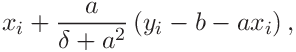
The solution is
![\displaystyle\frac{1}{2s_{xy}}\left[s_{yy}-\delta s_{xx}\pm\sqrt{(s_{yy}-%
\delta s_{xx})^{2}+4\delta s_{xy}^{2}}\right]](mi/mi326.png) |
(68) | ||||
| (69) | |||||
 |
(70) |
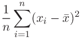
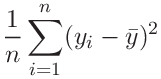
where
 |
(71) | ||||
 |
(72) | ||||
 |
(73) | ||||
 |
(74) | ||||
 |
(75) |
A.3 Least squares - 3/2 power fit
We seek the best fit
| (76) |
by minimizing the sum of (vertical) distances of datapoints from the curve
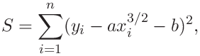 |
with respect to the parameters ![]() ,
, ![]() .
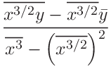
The solution is
.
The solution is
 |
(77) | ||||
| (78) |
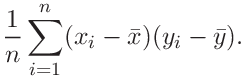
where
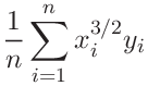 |
(79) | ||||
 |
(80) | ||||
 |
(81) | ||||
|
(82) |
![[LOGO]](data:image/png;base64,iVBORw0KGgoAAAANSUhEUgAAAAsAAAAOCAYAAAD5YeaVAAAAAXNSR0IArs4c6QAAAAZiS0dEAP8A/wD/oL2nkwAAAAlwSFlzAAALEwAACxMBAJqcGAAAAAd0SU1FB9wKExQZLWTEaOUAAAAddEVYdENvbW1lbnQAQ3JlYXRlZCB3aXRoIFRoZSBHSU1Q72QlbgAAAdpJREFUKM9tkL+L2nAARz9fPZNCKFapUn8kyI0e4iRHSR1Kb8ng0lJw6FYHFwv2LwhOpcWxTjeUunYqOmqd6hEoRDhtDWdA8ApRYsSUCDHNt5ul13vz4w0vWCgUnnEc975arX6ORqN3VqtVZbfbTQC4uEHANM3jSqXymFI6yWazP2KxWAXAL9zCUa1Wy2tXVxheKA9YNoR8Pt+aTqe4FVVVvz05O6MBhqUIBGk8Hn8HAOVy+T+XLJfLS4ZhTiRJgqIoVBRFIoric47jPnmeB1mW/9rr9ZpSSn3Lsmir1fJZlqWlUonKsvwWwD8ymc/nXwVBeLjf7xEKhdBut9Hr9WgmkyGEkJwsy5eHG5vN5g0AKIoCAEgkEkin0wQAfN9/cXPdheu6P33fBwB4ngcAcByHJpPJl+fn54mD3Gg0NrquXxeLRQAAwzAYj8cwTZPwPH9/sVg8PXweDAauqqr2cDjEer1GJBLBZDJBs9mE4zjwfZ85lAGg2+06hmGgXq+j3+/DsixYlgVN03a9Xu8jgCNCyIegIAgx13Vfd7vdu+FweG8YRkjXdWy329+dTgeSJD3ieZ7RNO0VAXAPwDEAO5VKndi2fWrb9jWl9Esul6PZbDY9Go1OZ7PZ9z/lyuD3OozU2wAAAABJRU5ErkJggg==)